Western Australian Branch SSA Meeting article October 2019
Dr John Henstridge (Chief Statistician and Managing Director of Data Analysis Australia) spoke on “Presenting Uncertainty and Risk” at the WA Branch meeting on Tuesday 8th October 2019. This was held in the Cheryl Praeger lecture theatre (named after John’s wife) at the University of Western Australia. He outlined areas where uncertainty is often misunderstood by non-statisticians and gave suggestions for statisticians to more effectively communicate uncertainty to non-statisticians.
John based his talk around work performed for a client that presented challenges as how to report uncertainty and risk. He outlined that most statistics is performed for the benefit of non-statisticians; while statisticians are good at handling uncertainty, many non-statisticians are not and may assume statistical methods give certainty. It is up to statisticians to communicate uncertainty clearly to others.
In official publications, data is often presented as fact where the uncertainty is unquantified. This approach is often seen in accounting, where immaterial differences are allowed, when it “doesn’t make much difference” to the overall data. There may be uncertainty to the underlying mechanism giving rise to the numbers, but not the numbers themselves.
In some areas, it is argued that “there are too many numbers” such that it is impractical to represent the uncertainty. John stated the in reality this view is wrong, and uncertainty can be dealt with regardless of the complexity of the data. Where data can be generated, then you can almost always provide uncertainty estimates using bootstrap methods. John gave an example where he’d worked on the Western Australian Travel Survey. A jackknife (instead of the bootstrap for technical reasons) had been performed on the estimates produced by an automated report, where 10 sub-sampled reports were compared character-by-character to generate standard-errors. This was an extreme case, and not one he might suggest in the future, but it does illustrate that bootstrapped standard errors are virtually always possible. The issue is what to present and how to present it.
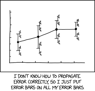
John then gave a brief history of error bars. Error bars have their origin in metrology (the science of measurement [1]) that interprets them as absolute limits, that is, the true value is always within the error bars. Statisticians later appropriated error bars, where they usually denote confidence intervals. Confidence intervals exist for mathematical convenience but are misinterpreted by most users. He suggested it would be worthwhile for statisticians to read standard texts from international metrology organisations.

In some publications it’s not always clear how this uncertainty displayed in error bars is derived. Examples were provided where the numbers were certain, but error bars were provided. When uncertainty is given without stating what the model is, it’s hard to know if the uncertainty has been calculated correctly.
Next, John questioned the practice of presenting an interval when we don’t mean it. While error bars have been borrowed from metrology, statisticians rarely think of error bars as giving the full variation, with the true value allowed to lie outside of the interval. When John Tukey invented boxplots, technological limitations enforced vertical and horizontal lines. We now have access to other ways of presenting variation with diamond, violin, fan and density strips plots. John Henstridge prefers representing variation with violin plots as these give a better idea of the full distribution and are more robust to display and printing methods.
Related to this is the “p-value problem”, where uncertainty is interpreted with certainty. This is in part the fault of statisticians in not effectively communicating the appropriate interpretation of p-values. Too often, significant/not-significant p-values leads to strict cut offs on the truth of the result. Similarly, confidence intervals are frequently misunderstood to have the true value within the range. Statisticians have some responsibility for these misunderstandings.
The American Statistical Association [2] provided a statement in 2016 on p-values, and although John Henstridge said it was technically correct and provided lots of things not to do, it was not clear what we should do. He felt that the statement may have missed the point, trying to have a formalism when presenting the results of analysis when there is a deeper problem of how to represent uncertainty.
Finally, John strongly recommended statisticians read “Communicating uncertainty about facts, numbers and science” [3] from the Royal Society Open Science initiative. This has lots of useful information on both types of uncertainty and communicating uncertainty.
A recording of the seminar is available on the Branch Seminar Videos page.
John Henstridge is the Chief Statistician and Managing Director of Data Analysis Australia, a statistical consulting firm that he founded in 1988. While his original specialty was time series applied to signal processing problems, as a consultant statistician he has worked across many areas of statistics. He is an Accredited Statistician (of the Statistical Society of Australia) and a Chartered Statistician (of the Royal Statistical Society) and served as the national President of the Statistical Society of Australia between 2013 and 2016.
Rick Tankard
SSA WA Branch Secretary
References:
[1] See for example International Bureau of Weights and Measures or Bureau international des poids et mesures, https://www.bipm.org/en/publications/guides/#gum
[2] Wasserstein, Ronald L., and Nicole A. Lazar. "The ASA’s statement on p-values: context, process, and purpose." The American Statistician 70, no. 2 (2016): 129-133.
[3] van der Bles, Anne Marthe, Sander van der Linden, Alexandra LJ Freeman, James Mitchell, Ana B. Galvao, Lisa Zaval, and David J. Spiegelhalter. "Communicating uncertainty about facts, numbers and science." Royal Society open science 6, no. 5 (2019): 181870.
